Pivot Table Value Field Settings : Pivot Table Part 2 Grouping, Value field Setting, New ... - Once you add a field to a pivot table, you can view and change attributes of the field using the field settings dialog box.. Start building the pivot table to add the text to the values area, you have to create a new special kind of calculated field called a measure. Or while having a value selected, you can go to pivottable tools > analyze > active field > field settings you now have your value field settings! Then, in the value field settings dialog box, click the number format button and apply the format you want. Refresh the pivot table (keyboard shortcut: It's not as simple as clicking the drop down arrow in the values section, selecting value field settings and selecting median as median does not exist as an option… in fact you can't actually display the median in a pivot table.
Select a field in the values area for which you want to change the summary function in the pivot table, and right click to choose value field settings, see screenshot: Select value field settings > show values as > number format > percentage. To access value fields settings, right click on any value field in the pivot table. By default pivot table takes sum for number field, and count for text filed. Drag events to the row field.
How To Create A Pivot Table In Excel - An Easy Guide from tinytutes.com The calc column depicts the type of calculation and there is a serial number for each. The total will be changed to a custom calculation, to show the percentage for each region's sales of an item, compared to the sales grand total for all items. To change the type of calculation we need to use value field settings in pivot table. This video gives you a brief introduction to the value field settings in a pivot table. Consider this data & a pivot table! The standard deviations shown in the pivot table are the same as those that were calculated on the worksheet. And we create a simple pivot from this data set. A list of options will be displayed.
Subtotals appear at the top of each group instead of the bottom.
A pivottable with the sum function as the default will be created. The variances shown in the pivot table are the same as those that were calculated on the worksheet. Another way to access value field settings is the area where we drop fields for the pivot table. In this example, the pivot table has item in the row area, region in the column area, and units in the values area. This video gives you a brief introduction to the value field settings in a pivot table. The calc column depicts the type of calculation and there is a serial number for each. Select a field in the values area for which you want to change the summary function in the pivot table, and right click to choose value field settings, see screenshot: Then, in the value field settings dialog box, click the number format button and apply the format you want. 30 pivot table tricks | basic to advanced | pivot table course: If summary functions and custom calculations do not provide the results that you want, you can create your own formulas in calculated fields and calculated items. Go to pivottable fields > values> value field settings you can also right click on a value and select value field settings. To access value field settings, right click on any value field in the pivot table. Refresh the pivot table (keyboard shortcut:
Pivot table stddevp summary function. Select a field in the values area for which you want to change the summary function in the pivot table, and right click to choose value field settings, see screenshot: Select the cells that contain the values we want to format (j3:j7), and in the lower right portion of the pivottable field list, under values, click sum of sales. The value field settings dialog box is displayed. However, if a pivottable was set up with blank cells in the source data, the default for products sales would have been count instead of sum.
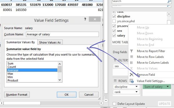
23 things you should know about Excel pivot tables | Exceljet from exceljet.net A list of options will be displayed. In the value field settings dialog box, select average in the summarize value field by list under summarize values by tab, rename the field name as median (there is space before median) in the custom name box, and click the ok button. 30 pivot table tricks | basic to advanced | pivot table course: Subtotals appear at the top of each group instead of the bottom. Another way to access value field settings is the area where we drop fields for the pivot table. With values field settings, you can set the calculation type in your pivottable. Name, winand fx % of wins to the values field. The source name is the name of the field in the data source.
Select value field settings > show values as > number format > percentage.
30 pivot table tricks | basic to advanced | pivot table course: Consider this data & a pivot table! Start building the pivot table to add the text to the values area, you have to create a new special kind of calculated field called a measure. Look at the top of the pivot table fields list for the table name. The value field settings dialog box is displayed. A pivottable with the sum function as the default will be created. Refresh the pivot table (keyboard shortcut: In this example, the pivot table has item in the row area, region in the column area, and units in the values area. However, if a pivottable was set up with blank cells in the source data, the default for products sales would have been count instead of sum. Pivot table varp summary function. A list of options will be displayed. Subtotals appear at the top of each group instead of the bottom. The calc column depicts the type of calculation and there is a serial number for each.
Select count function in the summarize value field by list box, and click ok button. In the end of the list (most 3rd from last) you will see value field settings. The calc column depicts the type of calculation and there is a serial number for each. To access value field settings, right click on any value field in the pivot table. The standard deviations shown in the pivot table are the same as those that were calculated on the worksheet.
How to Use Pivot Table Field Settings and Value Field Setting from www.exceltip.com In this example, the pivot table has item in the row area, region in the column area, and units in the values area. In the value field settings dialog box, select average in the summarize value field by list under summarize values by tab, rename the field name as median (there is space before median) in the custom name box, and click the ok button. Select the cells that contain the values we want to format (j3:j7), and in the lower right portion of the pivottable field list, under values, click sum of sales. In the end of the list (most 3rd from last) you will see value field settings. Add the field to the values area of the pivot table. Then, in the value field settings dialog box, click the number format button and apply the format you want. Select count function in the summarize value field by list box, and click ok button. Drag events to the row field.
In the resulting pivot table worksheet, expand table1 in the pivottable fields menu on the right.
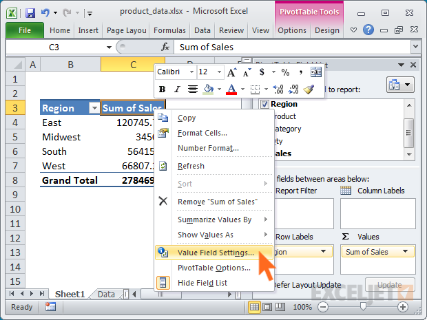
Right click on sum of revenue column and click on value field settings… And we create a simple pivot from this data set. Select value field settings > show values as > number format > percentage. However, if a pivottable was set up with blank cells in the source data, the default for products sales would have been count instead of sum. Select the cells that contain the values we want to format (j3:j7), and in the lower right portion of the pivottable field list, under values, click sum of sales. Then in the value field settings dialog box, select one type of calculate which you want to use under the summarize value by tab, see screenshot: Add the field to the values area of the pivot table. To use the varp summary function, when the qty field is added to the pivot table, change the summary calculation to varp. Look at the top of the pivot table fields list for the table name. You can also decide on how you want to display your values. In the value field settings dialog box, select average in the summarize value field by list under summarize values by tab, rename the field name as median (there is space before median) in the custom name box, and click the ok button. On the analyze tab, in the active field group, click active field, and then click field settings. Multiple fields in the rows area are all collapsed into column a with a generic heading of row labels. empty cells appear in the pivot table as blank instead of zero.